Phaser Coding Tips 8 "Sprite Motion Paths Tutorial" Revisited, Part 1
- cedarcantab
- Mar 28, 2022
- 12 min read
When creating shoot-em-ups, you want to have enemies flying in different patterns. You can certainly get sophisticated patterns by using trigonometry. Sometimes it's useful to be able to the enemies fly along customised motion paths based on splines. I set out to study different ways of moving enemies in different pattern, first by looking at a Phaser 2 tutorial by the great Richard Davey titled "Sprite Motion Paths Tutorial" available here, and this post is a document of my learnings.
The tutorial is from 2 March 2015 and is based on Phaser 2.
Phaser 3 can achieve the same effects but in more compact ways. Not only that Phaser 3 offers much "higher" functionality/methods. Nevertheless, it is interesting to work through the original tutorial as it is helpful (and just interesting) to understand some of the "nuts-and-bolts".
First, my Phaser 3 conversion of the original tutorial code is below.
Original tutorial - it's about different ways of Interpolation between points
The tutorial talks about 3 methods of the Phaser.Math class (which, as far as I can tell, exist unchanged in Phaser 3):
linearInterpolation
bezierInterpolation
catmullRomInterpolation.
All the methods take 2 parameters:
parameter v: the first being an array of numbers to interpolate through, and
paramter t: second parameter is how far along you want to interpolate (being a number between 0 and 1).
So, replicating the example from the original tutorial in Phaser 3 like so, gives 320, half-way between 0 and 640
var points = [ 0, 128, 256, 384, 512, 640 ];
var distance = 0.5;
var result = Phaser.Math.Interpolation.Linear(points, distance);
Linear Interpolation
Now, linear interpolation (sometimes referred to as lerp, from linear interpolation) is easiest to understand in terms of 2 points (I refer to "points", because, although we are talking about interpolating between 2 numbers, it is easier to understand the idea of interpolation with points in 2D space). Imagine there are 2 points p0 and p1, and you have a third point somewhere in between. In linear interpolation, all you are doing is to join p0 and p1 with a straight line, and the third point is a point that lies on that line. Typically you talk about interpolations in terms of the t-value which ranges from 0 to 1, kind of like a percentage. If t is 0, the interpolated point is at p0, and when t is at 1, it is at p1. Conceptually, the interpolated value is a weighted average of p0 and p1, as confirmed by the formula is as follows.
(1-t) * p0 + t * p1 = (p1 - p0) * t + p0And in fact, that is exactly what Phaser.Math.Interpolation.Linear does. It loops through all the points passed in the v parameter, calling the Phaser.Math.Linear function, which, if you look under the Phaser hood looks like below:
var Linear = function (p0, p1, t)
{
    return (p1 - p0) * t + p0;
};
But the beauty of the Phaser.Math.Interpolation.Linear method is that you can feed it more than 2 numbers, and the method will work out which p0 and p1 points (as well as the "t" adjusted to fit between p0 and p1) should be fed to the Phaser.Math.Linear method.
It is described in plenty of detail in this wikipedia here (also referenced by the official Phaser document).
Specifically, it picks p0 and p1 by looking at how many points are passed, and taking the two points "around" the t, by means of the following code, with m being index for p0 (in the example, it would be 2, or 3rd item in array) and i+1 being p1. The "adjusted" t to be passed to the underlying Phaser.Math.Linear method is calculated as f - i (in the example, it would be (6-1)*0.5 - floor((6-1)*0.5) = 0.5; ie it is taking the mid-point between 256 and 384 = 320.
var m = v.length - 1;
var f = m * k;
var i = Math.floor(f);
t of 0.5 is not necessarily the mid-point of the 1st point and the last point of v
Note that in the the above, it is taking the mid-point between the 3rd and 4th points, not the middle of the 1st and the last points. If the 3rd and 4th points were "buched" towards one end of the series of points, it would not result in 320. As we will see later, it is important to be cognisant of this.
Bezier Curve
Things suddenly become much more...mathematical with Bezier curves. The wikipedia page here gives a relatively easy to understand high level overview of what this is about.
In fact, Bezier curve can be thought of as an extension of the linear interpolation of the above (when there is only 2 points, the Bezier curve is the same as the linear "curve" above). In the case of the quadractic bezier curve (3 points), what you are doing is (i) lerp by the same t-value between p0-p1, and p1-p2, then join the 2 lerped points, and (ii) lerp between the 2 newly created points by the same t-value, that is what quadractic Bezier curve is about. This Desmos graph makes it very clear graphically what is happening (except it uses k whereas I have referred to t-value).
The Phaser.Math.Interpolation.Bezier(v, k) goes straight into interpolating across n number of points, and the mathematics increasingly look frightening as the number of points increase, the concept of iteratively lerping remains the same. Just to prove my point below goes into a bit more detail about bezier curves with 3 points (quadractic Bezier) and 4 points (cubic bezier).
Quadratic Bezier
Wiki gives the following expression:

As explained above, bezier curves are based on nesting of lerps. So, if we call the interpolated points between p0-p1 and p1-p2, A and B respectively, and the interpolated point P (the final interpolation target) between A and B, we can expressed as below (De Casteljau's algorithm):
A = lerp(t, p0, p1) = (1-t)*p0 + t*p1
B = lerp(t, p1, p2) = (1-t)*p1 + t*p2
P = lerp(t, A, B) = (1-t) * A + t* B
= (1-t) * ((1-t)*p0 + t*p1) + t * ((1-t)*p1 + t*p2)
= (1-t) * (1-t) * p0 + (1-t) * t * p1+ t * (1-t) * p1 + t * t * p1
= (1-t)^2 * p0 + 2*t*(1-t)*p1 + t^2*p2
Voila! Same as the Wikipedia formula!
There is a method to interpolate in this manner: Phaser.Math.Interpolation.QuadraticBezier(t, p0, p1, p2). And indeed, if you look under the hood, the actual code (at least the body of it) is as follows. P0, P1, P2 are defined as methods that correspond exactly to the above equation.
var QuadraticBezierInterpolation = function (t, p0, p1, p2)
{
    return P0(t, p0) + P1(t, p1) + P2(t, p2);
};
Cubic Bezier
When there are 4 points it becomes a Cubic Bezier Curve, and as expected, there is a method for this: Phaser.Math.Interpolation.CubicBezier(t, p0, p1, p2, p3). Again, taking the above approach, cubic Bezier can be expressed as:
A = lerp(t, p0, p1) = (1-t)*p0 + t*p1
B = lerp(t, p1, p2) = (1-t)*p1 + t*p2
C = lerp(t, p2, p3) = (1-t)*p2 + t*p3
D = lerp(t, A, B) = (1-t)*A + t*B
E = lerp(t, B, C) = (1-t)*C + t*C
P = lerp(t, D, E) = (1-t)*D + t*E
which in turn graphically can be thought of as below.
If you work throught the maths for P above, it can be expanded to:
P = -t^3*p0 + 3*t^2*p0-3*t*p0 + p0
+ 3*t^3*p1- 6 *t^2*p1+3*t*p1
- 3*t^3*p2 +3*t^2*p2
+ t^3*p3
And re-arranging it a bit more gives below, where the points are factored out and "weighted" by polynomials.
P = p0*(-t^3+3*t^2-3*t-1)
+ p1*(3*t^3-6*t^2+3*t)
+ p2* (-3*t^3 + 3* t^2)
+ p3* t^3
which is called the Bernsein Polynomial Form of the Bezier curve.
By expressing the formula with the points factored out, those of you with a mathematical bent will realise you can start getting various properties of the Bezier curve by taking derivatives of the above (but that is beyond my capability to explain).
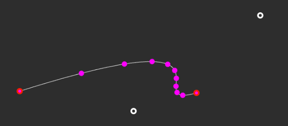
I will mention at one important characteristic of the t-value; namely that linearly increasing the t from 0 to 1 does not mean the interpolated point moves "linearly" across the resulting Bezier curve. This is clearly illustrated with the following where the purple dots have been plotted by incrementing t from 0 to 1 by 0.1 intervals (ie 10 segments, 11 points).
How long is a piece of Bezier curve?
In fact, there is no mathematical formula to calculate the "length" of a Bezier curve. For game programmers though where absolute accuracy is not required one can estimate the length of the curve by dividing the curve into little segments, calculating the length of the sub-segments pretending they are straight lines and adding them up. The smaller the sub-segments are, the more "accurate" the estimate becomes, although of course computationally more expensive. I believe that the arcLengthDivisions and cacheArcLengths properties and the getLengths([divisions]) method of the Phaser.Curves.CubicBezier class are related to this.
Since it's computationally expensive, you can go through the process of splitting the curve into small pieces, and generate a look-up table and store the distance along the curve, with its corresponding t-value. Once such a look-up table is created, you can work backwards and get the (approximate) t-value corresponding to a particular distance. This is apparently referred to as Arc Length Parameterisation. And indeed, Phaser provides a method to do just that: getTFromDistance(distance, [divisions])
Bezier curves of degree-n
The method used in the example - Phaser.Math.Interpolation.Bezier(v, k) - can take more than 4 points as an array. The wiki gives the following definition for Bezier curves of degree-n as follows

where bits that are being sumed (expanded below) are known as Bernstein basis polynomials of degree n.

where t0 = 1, (1 − t)0 = 1, and that the binomial coefficient is:

and indeed, looking at the underlying code of the actual Phaser.Math.Interpolation.Bezier(v, k) method is as below:
var BezierInterpolation = function (v, k) {
    var b = 0;
    var n = v.length - 1;
    for (var i = 0; i <= n; i++) {
        b += Math.pow(1 - k, n - i) * Math.pow(k, i) * v[i] * Bernstein(n, i);
    }
    return b;
};
and the Phaser.Math.Bernstein method is as follows:
var Bernstein = function (n, i)
{
    return Factorial(n) / Factorial(i) / Factorial(n - i);
};
As can be seen with the example, a distinguishing feature of the Bezier curve is that the curve does not pass through all the points but the control points influence the shape of the curve. Hence you will definitely need to use some kind of graphical utility to create exactly the curve you want.
CatmullRom
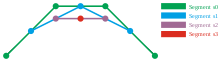
The original tutorial then uses another method called Phaser.Math.Interpolation.CatmullRom to draw the spline. The original tutorial refers to an article here, which is short but informative. The site explains that "To calculate a point on the curve, two points on either side of the desired point are required, as shown on the left. The point is specified by a value t that signifies the portion of the distance between the two nearest control points", referring to the following image:

The site then goes on to explain the mathematics behind the curve fitting. To my simple mind, I think of it like this. We are generating a curve between control points p1 and p2, with p0 and p3 as additional control points that guide at what angle the curve should be going through points p1 and p2. To find a particular interpolated point along the spline, t is used, which starts at 0 at p1, and end at 1 at p2; ie to draw the curve from p1 to p2, t is incremented from 0 to 1 in small incremenets, repeatedly calculating the interpolated point. In CatmullRom interpolation, each point "influence" the interpolated point. Conceptually, as t approaches p2, the interpolated point is more infleucend by p2 and less influenced by p1 (or the interpolated point in middle of p1 and p2 is equally influenced). At p2 the interpolated point is 100% influeced by p2, ie the point is on p2 itself. Control points p0 and p3 also influence the interpolated point - if they didn't, the interpolation would be just a straight line between p1 and p2. p0 and p3 kind of "repel" the interpolated point, so looking at the picture above, p0 would tend to push the interpolated point below the straight line between p1 and p2, whereas p3 would tend to push the point above the straight line between p1 and p2.
The site goes onto to say (after giving an explanation of the mathematics):
While a spline segment is defined using four control points, a spline may have any number of additional control points. This results in a continuous chain of segments, each defined by the two control points that form the endpoints of the segments, plus an additional control point on either side of the endpoints. Thus for a given segment with endpoints Pn and Pn+1, the segment would be calculated using [Pn-1, Pn, Pn+1, Pn+2].
In other words, rather like the linear interpolation method, whilst we can feed an array of n points to this method, Phaser is actually looping through the points (4 points at a time), calculating CatmullRom splines between each of the control points. This "cycling" is similar to the method described above for Linear interpolation; the implication being that moving t=0.5 does not necessarily mean the "mid point" between the 1st and the last point.
Needless to say, from the game coder's perspective the biggest difference of the CatmullRom vs the Bezier curve is that the curve actually goes through all the control points.
In addition, as we will see later, Phaser 3's spline method is based on CatmullRom interpolation as opposed to Bezier interpolation.
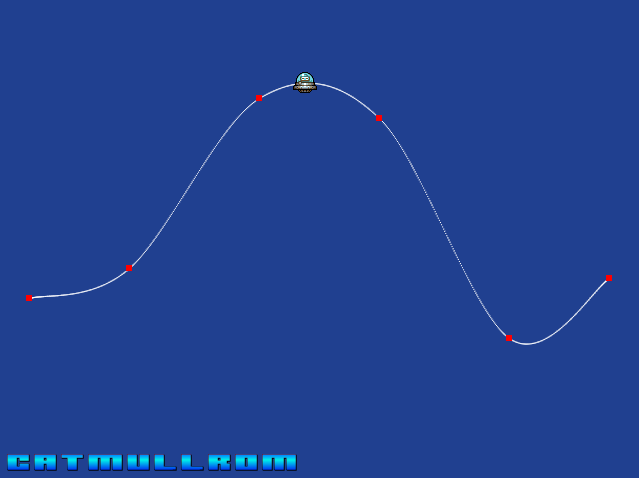
Splines and Motion Paths
The tutorial example code uses the above interpolation methods to create an array (called this.path) of 640 "points" (640 simply being the number of pixels across the width of the screen), along which to move an alien UFO. In effect, the alien is moved along the "motion path" by sequentially setting its x/y coordinates according to the 640 "points" data held in this array (or "spline").
Along the way the "rotation" of the sprite is also calculated by reference to the angle between the "current" point on the spline, and the "previous" point, like so. This is in effect gives the "approximate" tangent of the path.
let node = { x: px, y: py, angle: 0 };
  if (ix > 0) {
    node.angle = Phaser.Math.Angle.BetweenPoints(this.path[ix - 1], node);
  }
This resetting of x/y coordinate and the angle of the sprite is done from the update method.
The speed of the alien
What this means is that every refresh (typically 1/60 second) the alien moves along "one point". There are 640 points from the beginning to the end of the "path" so to complete the path takes 640 x (1/60) = 10.67 seconds.
  update(time, delta) {
    this.alien.setPosition(this.path[this.pi].x, this.path[this.pi].y)
    this.alien.rotation = this.path[this.pi].angle;
    this.pi++;
    if (this.pi >= this.path.length) this.pi = 0;
  }
What if you wanted to change the speed at which the alien moved? One simple way would be to change the number of "points" on the spline, which in the above example is set at 640 points. If you reduced the number of points, the alien would move after. If increased, the alien would move slower.
Using number Tweens to control the "time" to traverse the path
The tutorial example pre-calculated x/y coordinates along the spline and held it in an array and cycled through the pre-calculated array, and cycle through that from the game update loop.
Instead of pre-calculating "every point" on the spline at fixed intervals, you could theoretically calculate the "next point" every that it is needed. If you used a tween to calculate the point, you would not be tied to the speed of the update cycle.
(I am not necessarily suggesting that this is a great way to do things, but only as a way to introduce a way to move sprites along a spline using tweens, as a precursor to path follower objects to be explored subsequently posts).
For example, you could use the following number tween to change a "t-value" from 0 to 1 over 5 seconds.
    this.moveTween = this.tweens.addCounter({
      from: 0,
      to: 1,
      duration: 5000,
      repeat: -1
    });
Then you could get the "next point" base on the t-value with the following code.
 update(time, delta) {
    this.pi = this.moveTween.getValue();
    const px =  Phaser.Math.Interpolation.CatmullRom(this.points.x, this.pi);
    const py =  Phaser.Math.Interpolation.CatmullRom(this.points.y, this.pi);
    this.alien.setPosition(px, py)
  }
Although not directly controlling the velocity as such, one can set the time taken to travel the entire motion path. In order to make the alien face the direction of the path, you need to calculate the tangent of the path in the same way as the first example code, only this time you need to do it every refresh rather than have the angles pre-calculated.
The slight worry with the above is that I am now having Phaser go through the CatmullRom calculation every refresh to calculate the position, as opposed to pre-calculating all of the positions.
Another way to do it via tweens
Whilst Phaser 3 tweens cannot target primitives, it can target pretty much any object as far as I am aware. Hence exactly the same effect as the above can be achieved by creating the following tween (ignore the second element in this.path object - it is not used in this example, but is a prelude to the next post on Phaser 3 splines).
    this.path = { t: 0, vec: new Phaser.Math.Vector2()};
    this.tweens.add({
        targets: this.path,
        t: 1,
        ease: 'Linear',
        duration: 5000,
        repeat: -1
    });
and changing the code in the update function as follows.
const px =  Phaser.Math.Interpolation.CatmullRom(this.points.x, this.path.t);
const py =  Phaser.Math.Interpolation.CatmullRom(this.points.y, this.path.t);

this.alien.setPosition(px, py)
You will notice that the alien seems to speed up as it "climbs up" the long stretch, and "climbs down" the long stretch, despite t being incremented in a linear manner. This is because of the way the interpolation works across multiple control points, as described above.
The Number Tween code example is not the recommended way
As I said, I mention the above as a prelude to the Phaser 3 path follower object which, in principle (not exactly), is based on the logic above - hence for users of Phaser 3, the above is not the recommended way of moving objects along a motion path.
Nevertheless, if anyone is interested in playing around with the above that uses the counter tween, it is in the Codepen below (just the CatmullRom).
Useful references


Comments